For this activity, we classify the same set of objects as with activities 18 and 19 but using neural networks instead. A neural network will have three parts, the input layer, the hidden layer and the output layer. For classification purposes, the input layer contains the features and the output would contain the classes. As with activity 19 I used piatos and pillows as my 2 classes. The output may either be 0 (piatos) or 1 (pillows) depending on which class a sample belongs.
The code below follows the one written by Jeric. I used 4 input layer neurons, 8 hidden layer neurons and 1 output layer neuron. The following is the code I used, the training and test sets are the ones in activity 19.
-----------------------------------------------------------------------------------
chdir("C:\Users\RAFAEL JACULBIA\Documents\subjects\186\activity20");
N = [4,8,1];
train = fscanfMat("train.txt")';// Training Set
t = [0 0 0 0 1 1 1 1];
lp = [2.5,0];
W = ann_FF_init(N);
T = 500; //Training cyles
W = ann_FF_Std_online(train,t,N,W,lp,T);
test = fscanfMat("test2.txt")';
class = ann_FF_run(test,N,W)
round(class)
--------------------------------------------------------------------------
The following are the outputs of the program :
0.0723331 0.0343279 0.0358914 0.0102084 0.9948734 0.9865080 0.9895211 0.9913624
After rounding off, we see that the above outputs are 100% accurate.
I grade myself 10/10 for again getting a perfect classification. Thanks to jeric for the code and to ed for his help.
Thursday, October 9, 2008
Thursday, October 2, 2008
Activity 19: Probabilistic Classification
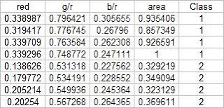
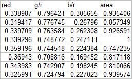
In this activity, we again classify different objects like what we did in activity 18. Only this time we perform linear discrimination analysis. It mainly assumes that our classes are separable by a linear combination of different features of the class. Class membership is attained for when a certain sample has minimum error of classification. A detailed discussion is given in Linear_Discrimant_Analysis_2.pdf by Dr. Sheila Marcos. The samples I used for this activity are piatos(class 1) and pillows (class 2). The features I used are: normalized area obtained via pixel counting, average value of the red component, ratio of the average value of the green component to the red component, and the ratio of the average value of the blue component to the red component. These parameters are obtained using the procedure described in my earlier post for activity 18. The first four samples are used as training set and the last four are used as the test set.
Using the above training set and the methods described in the provided pdf file, we can compute for the covariance matrix given below:
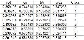
The test set is given below:
From this test set, the computed discrimant values are:
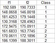 From these result it is obvious that I was able to obtain a 100% correct classification. I also tried this with a different sample combination (pillows vs squidballs) and I still got 100% correct classification. The following is the code I used:
-----------------------------------------------------------------------
chdir("C:\Users\RAFAEL JACULBIA\Documents\subjects\186\activity19");
x = [];
y = [];
x1 = [];
x2 = [];
u1 = [];
u2 = [];
x1o = [];
x2o = [];
c1 = [];
c2 = [];
C = [];
n = 8;
n1 = 4;
n2 = 4;
x = fscanfMat("x.txt");
y = fscanfMat("y.txt");
test = fscanfMat("test.txt");
x1 = x(1:n1,:);
x2 = x(n1+1:n,:);
u1 = mean(x1,'r');
u2 = mean(x2,'r');
u = mean(x,'r');
x1o(:,1) = x1(:,1) - u(:,1);
x1o(:,2) = x1(:,2) - u(:,2);
x1o(:,3) = x1(:,3) - u(:,3);
x1o(:,4) = x1(:,4) - u(:,4);
x2o(:,1) = x2(:,1) - u(:,1);
x2o(:,2) = x2(:,2) - u(:,2);
x2o(:,3) = x2(:,3) - u(:,3);
x2o(:,4) = x2(:,4) - u(:,4);
c1 = (x1o'*x1o)/n1;
c2 = (x2o'*x2o)/n2;
C = (n1/n)*c1 + (n2/n)*c2;
p = [n1/n;n2/n];
class = [];
for i = 1:size(test,1)
f1(i) = u1*inv(C)*test(i,:)'-0.5*u1*inv(C)*u1'+log(p(1));
f2(i) = u2*inv(C)*test(i,:)'-0.5*u2*inv(C)*u2'+log(p(2));
end
f1-f2
------------------------------------------------------------------------
I proudly grade myself 10/10 for getting it perfectly without the help of others. I also consider this activity one of the easiest because of the step by step method given in the provided file.

Using the above training set and the methods described in the provided pdf file, we can compute for the covariance matrix given below:
0.0062310 0.0087568 0.0012735 0.0226916
0.0087568 0.0129916 0.0019430 0.0329768
0.0012735 0.0019430 0.0005591 0.0042263
0.0226916 0.0329768 0.0042263 0.0876073
The test set is given below:

From this test set, the computed discrimant values are:
 From these result it is obvious that I was able to obtain a 100% correct classification. I also tried this with a different sample combination (pillows vs squidballs) and I still got 100% correct classification. The following is the code I used:
-----------------------------------------------------------------------
chdir("C:\Users\RAFAEL JACULBIA\Documents\subjects\186\activity19");
x = [];
y = [];
x1 = [];
x2 = [];
u1 = [];
u2 = [];
x1o = [];
x2o = [];
c1 = [];
c2 = [];
C = [];
n = 8;
n1 = 4;
n2 = 4;
x = fscanfMat("x.txt");
y = fscanfMat("y.txt");
test = fscanfMat("test.txt");
x1 = x(1:n1,:);
x2 = x(n1+1:n,:);
u1 = mean(x1,'r');
u2 = mean(x2,'r');
u = mean(x,'r');
x1o(:,1) = x1(:,1) - u(:,1);
x1o(:,2) = x1(:,2) - u(:,2);
x1o(:,3) = x1(:,3) - u(:,3);
x1o(:,4) = x1(:,4) - u(:,4);
x2o(:,1) = x2(:,1) - u(:,1);
x2o(:,2) = x2(:,2) - u(:,2);
x2o(:,3) = x2(:,3) - u(:,3);
x2o(:,4) = x2(:,4) - u(:,4);
c1 = (x1o'*x1o)/n1;
c2 = (x2o'*x2o)/n2;
C = (n1/n)*c1 + (n2/n)*c2;
p = [n1/n;n2/n];
class = [];
for i = 1:size(test,1)
f1(i) = u1*inv(C)*test(i,:)'-0.5*u1*inv(C)*u1'+log(p(1));
f2(i) = u2*inv(C)*test(i,:)'-0.5*u2*inv(C)*u2'+log(p(2));
end
f1-f2
------------------------------------------------------------------------
I proudly grade myself 10/10 for getting it perfectly without the help of others. I also consider this activity one of the easiest because of the step by step method given in the provided file.
Activity 18: Pattern Recognition
In this activity we are to identify to what class an object belongs to. We do this by extracting relevant features about different samples of the object and comparing its features to a training set. The criteria for membership in a certain class is when its features has a minimum distance to a certain class' representative features obtained by getting the mean of each features of the samples from each class. The classes I used are piatos chips, pillow chocolate filled snack, kwek kwek and squidballs. The images of the objects are shown below:
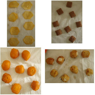
I chose four features that can be extracted from the objects; normalized area obtained via pixel counting, average value of the red component, ratio of the average value of the green component to the red component, and the ratio of the average value of the blue component to the red component. Since we have only eight samples I used the first four as a training set and the tested the class membership of the training set. The mean feature vectors are shown below:
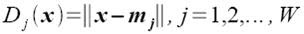
Class membership is obtained by taking the minimum distance between a test's feature to the mean of each feature, following the formula given by Dr. Soriano's pdf file:
Using the features and the above formula, I obtained 15 correct classifications out of 16 samples translating to a 93.75% correct classification.
For the extraction of the parameters of the samples, I performed parametric color image segmentation we learned from activity 16. Afterwards, I inverted the segmented image, performed the morphological closing operation and multiplied it to the original colored image to obtain a colored segmented image. I used excel to perform the minimum distance classification, it was tedious but I understand it better if I do it this way :0. The scilab code I used for the extraction of the parameters is shown below:
For this activity I grade myself 10/10 since I was able to get a relatively high correct classification percentage.
Ed David helped me a lot in this activity. Special thanks to Cole, JM, Billy, Mer, Benj for buying the samples for this activity.

I chose four features that can be extracted from the objects; normalized area obtained via pixel counting, average value of the red component, ratio of the average value of the green component to the red component, and the ratio of the average value of the blue component to the red component. Since we have only eight samples I used the first four as a training set and the tested the class membership of the training set. The mean feature vectors are shown below:

Class membership is obtained by taking the minimum distance between a test's feature to the mean of each feature, following the formula given by Dr. Soriano's pdf file:

Using the features and the above formula, I obtained 15 correct classifications out of 16 samples translating to a 93.75% correct classification.
For the extraction of the parameters of the samples, I performed parametric color image segmentation we learned from activity 16. Afterwards, I inverted the segmented image, performed the morphological closing operation and multiplied it to the original colored image to obtain a colored segmented image. I used excel to perform the minimum distance classification, it was tedious but I understand it better if I do it this way :0. The scilab code I used for the extraction of the parameters is shown below:
For this activity I grade myself 10/10 since I was able to get a relatively high correct classification percentage.
Ed David helped me a lot in this activity. Special thanks to Cole, JM, Billy, Mer, Benj for buying the samples for this activity.
Tuesday, September 16, 2008
Activity 17: Basic Video Processing
In this activity, we are to analyze a video clip. The video clip we will analyze is a simple kinematic experiment and we are to extract certain physical parameters of the experiment and confirm the results analytically. To analyze the video, we need to separate its frames then on this frames we can apply the image processing techniques we have learned so far in the course. The experiment we designed is a simple rolling disk on an inclined plane. An animated gif of the set of images is shown below (video was cropped before images were extracted).
Our goal is to extract the acceleration of the object along the incline. First, we need to segregate the region of interest (ROI) from the background. From our previous lessons, we have two choices of image segmentation, color and binary. Since the video does not really contain important color information, I chose to perform binary image segmentation. The crucial step in this method is the choice of the threshold value. For this activity I found that a threshold value of 0.6 produced good results. However, the a good segmentation was still not achieved since the reflection of light in some parts of the image caused the color of the ramp to be unequal. A gif image of the result after thresholding is shown below:

Clearly, this is not what we want so I performed opening operation using a 10x5 structuring element both to further segregate the ROI from the background of the image and to make the edges of the ROI smooth. The resulting set of images is shown below:
Now we can track the position of the ROI in time. The position over time in pixels can be obtained from the average value of the x pixel position per image. Distance per unit time where distance is in pixels and time is in frames. The conversion factor we obtained is 2mm/pixel and from the video the frame rate is 24.5fps. After conversion I was able to obtain 0.5428m/sec^2.
Analytically, from Tipler, the acceleration along an inclined plane of a hollow cylinder is given by a = (g*sin(theta))/2, where theta is the angle of the incline, for our case theta = 6degrees. Using the formula we get 0.5121m/sec^2. This translates to roughly 5.66% of error. The scilab code I used is given below:
------------------------------------------------------------------------------
chdir("C:\Users\RAFAEL JACULBIA\Documents\subjects\186\activity17\hollow");
I = [];
x = [];
y = [];
vs=[];
ys = [];
xs = [];
as=[];
se = ones(10,5);
se2 = im2bw(se2,0.5);
for i = 6:31
I = imread("hollow" + string(i-1) + ".jpg");
I = im2bw(I,0.6);
I = dilate(erode(I,se),se);
imwrite(I , string(i)+ ".png" );
I = imread( string(i) + ".png");
[x,y] = find(I==1);
xs(i) = mean(x);
ys(i) = mean(y);
end
ys = ys*2*10**(-3);
vs = (ys(2:25)-ys(1:24))*24.5;
as = (vs(2:24)-vs(1:23))*24.5;
-------------------------------------------------------------
I grade myself 9/10 for this activity for not getting a fairly high error percentage.
Collaborators:
Ed David
JM Presto

Our goal is to extract the acceleration of the object along the incline. First, we need to segregate the region of interest (ROI) from the background. From our previous lessons, we have two choices of image segmentation, color and binary. Since the video does not really contain important color information, I chose to perform binary image segmentation. The crucial step in this method is the choice of the threshold value. For this activity I found that a threshold value of 0.6 produced good results. However, the a good segmentation was still not achieved since the reflection of light in some parts of the image caused the color of the ramp to be unequal. A gif image of the result after thresholding is shown below:

Clearly, this is not what we want so I performed opening operation using a 10x5 structuring element both to further segregate the ROI from the background of the image and to make the edges of the ROI smooth. The resulting set of images is shown below:

Now we can track the position of the ROI in time. The position over time in pixels can be obtained from the average value of the x pixel position per image. Distance per unit time where distance is in pixels and time is in frames. The conversion factor we obtained is 2mm/pixel and from the video the frame rate is 24.5fps. After conversion I was able to obtain 0.5428m/sec^2.
Analytically, from Tipler, the acceleration along an inclined plane of a hollow cylinder is given by a = (g*sin(theta))/2, where theta is the angle of the incline, for our case theta = 6degrees. Using the formula we get 0.5121m/sec^2. This translates to roughly 5.66% of error. The scilab code I used is given below:
------------------------------------------------------------------------------
chdir("C:\Users\RAFAEL JACULBIA\Documents\subjects\186\activity17\hollow");
I = [];
x = [];
y = [];
vs=[];
ys = [];
xs = [];
as=[];
se = ones(10,5);
se2 = im2bw(se2,0.5);
for i = 6:31
I = imread("hollow" + string(i-1) + ".jpg");
I = im2bw(I,0.6);
I = dilate(erode(I,se),se);
imwrite(I , string(i)+ ".png" );
I = imread( string(i) + ".png");
[x,y] = find(I==1);
xs(i) = mean(x);
ys(i) = mean(y);
end
ys = ys*2*10**(-3);
vs = (ys(2:25)-ys(1:24))*24.5;
as = (vs(2:24)-vs(1:23))*24.5;
-------------------------------------------------------------
I grade myself 9/10 for this activity for not getting a fairly high error percentage.
Collaborators:
Ed David
JM Presto
Tuesday, September 2, 2008
Activity 16: Color Image Segmentation
The objective of this activity is to "segment" or select a region of interest from an image according to its color. To do this, we have to transform the RGB space into normalized chromaticity coordinates (NCC). We do this obtaining this by dividing each pixel by the sum of the RGB values in that pixel. Afterwards, the chromaticity can easily be represented by two color channels r and g since b = 1-r+g. The image used and the test image is shown below:
OBJECT

TEST IMAGE

Two methods are used in this activity, non-parametric and parametric. Parametric segmentation is done by determining the probability that a region belongs to the region of interest. In particular, a gaussian probability distribution function is assumed. For non-parametric segmentation, the frequency value of the pixel in the histogram itself is used to backproject the value for that pixel. The two dimensional histogram of the original image test image is shown below:
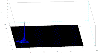 The x-axis corresponds to the R channel, the y-axis corresponds to the G channel and the z axis corresponds to the frequency. From the figure, it can be seen that the region where the frequency is highest is at the blue region as expected.
The following are the results of the color segmentation:
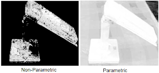 It can be seen from the images that parametric segmentation looks better as it was able to approximate the general shape of the blue parts of the lamp are well separated from the other colors. However, the non-parametric segmentation is very accurate in the sense that slight changes in the shade of blue in the image is no longer considered blue. This is easily observed in the post of the lamp since in this part the shade is darker than the top parts.
----------------------------------------------------------------------------------------------
----------------------------------------------------------------------------------------------
Scilab Codes:
Parametric
I = imread("lamp_section.jpg");
orig = imread("lamp_orig.jpg");
av = I(:,:,1)+I(:,:,2)+I(:,:,3);
r = I(:,:,1)./av;
g = I(:,:,2)./av;
b = I(:,:,3)./av;
av2 = orig(:,:,1)+orig(:,:,2)+orig(:,:,3);
r2 = orig(:,:,1)./av2;
g2 = orig(:,:,2)./av2;
b2 = orig(:,:,3)./av2;
r = r*255;
g = g*255;
frequency = zeros(256,256);
sizer = size(r);
for i=1:sizer(1)
for j=1:sizer(2)
x = abs(round(r(i,j)))+1;
y = abs(round(g(i,j)))+1;
frequency(x,y) = frequency(x,y)+1;
end
end
//imshow(log(frequency+0.0000000001));
r = r/255;
g = r/255;
mr = mean(r);
devr = stdev(r);
mg = mean(g);
devg = stdev(g);
pr = (1/(devr*sqrt(2*%pi)))*exp(-((r2-mr).^2)/2*devr);
pg = (1/(devg*sqrt(2*%pi)))*exp(-((g2-mg).^2)/2*devg);
prob = pr.*pg;
prob = prob/max(prob);
scf(0);imshow(orig);
scf(1);imshow(prob,[]);
-------------------------------------------------------------------------------------------------
Non Parametric:
I = imread("lamp_section.jpg");
orig = imread("lamp_orig.jpg");
sizeO = size(orig)
av = I(:,:,1)+I(:,:,2)+I(:,:,3);
r = I(:,:,1)./av;
g = I(:,:,2)./av;
b = I(:,:,3)./av;
av2 = orig(:,:,1)+orig(:,:,2)+orig(:,:,3);
r2 = orig(:,:,1)./av2;
g2 = orig(:,:,2)./av2;
b2 = orig(:,:,3)./av2;
r = r*255;
g = g*255;
frequency = zeros(256,256);
sizer = size(r);
for i=1:sizer(1)
for j=1:sizer(2)
x = abs(round(r(i,j)))+1;
y = round(g(i,j))+1;
frequency(x,y) = frequency(x,y)+1;
end
end
scf(0);imshow(log(frequency+0.0000000001));
r2 = r2*255;
g2 = g2*255;
seg = zeros(sizeO(1),sizeO(2));
sizer2 = size(r2);
for i = 1:sizer2(1)
for j = 1:sizer2(2)
x = abs(round(r2(i,j)))+1;
y = round(g2(i,j))+1;
seg(i,j) = frequency(x,y);
end
end
scf(1);imshow(log(seg+0.000000000001),[]);
scf(2);imshow(orig);
-------------------------------------------------------------------------------------------------
-------------------------------------------------------------------------------------------------
I will give myself a grade of 10 for this activity since the objectives were met and the results are interesting.
Collaborator:
Ed David


OBJECT

TEST IMAGE

 The x-axis corresponds to the R channel, the y-axis corresponds to the G channel and the z axis corresponds to the frequency. From the figure, it can be seen that the region where the frequency is highest is at the blue region as expected.
 The following are the results of the color segmentation:
 It can be seen from the images that parametric segmentation looks better as it was able to approximate the general shape of the blue parts of the lamp are well separated from the other colors. However, the non-parametric segmentation is very accurate in the sense that slight changes in the shade of blue in the image is no longer considered blue. This is easily observed in the post of the lamp since in this part the shade is darker than the top parts.
----------------------------------------------------------------------------------------------
----------------------------------------------------------------------------------------------
Scilab Codes:
Parametric
I = imread("lamp_section.jpg");
orig = imread("lamp_orig.jpg");
av = I(:,:,1)+I(:,:,2)+I(:,:,3);
r = I(:,:,1)./av;
g = I(:,:,2)./av;
b = I(:,:,3)./av;
av2 = orig(:,:,1)+orig(:,:,2)+orig(:,:,3);
r2 = orig(:,:,1)./av2;
g2 = orig(:,:,2)./av2;
b2 = orig(:,:,3)./av2;
r = r*255;
g = g*255;
frequency = zeros(256,256);
sizer = size(r);
for i=1:sizer(1)
for j=1:sizer(2)
x = abs(round(r(i,j)))+1;
y = abs(round(g(i,j)))+1;
frequency(x,y) = frequency(x,y)+1;
end
end
//imshow(log(frequency+0.0000000001));
r = r/255;
g = r/255;
mr = mean(r);
devr = stdev(r);
mg = mean(g);
devg = stdev(g);
pr = (1/(devr*sqrt(2*%pi)))*exp(-((r2-mr).^2)/2*devr);
pg = (1/(devg*sqrt(2*%pi)))*exp(-((g2-mg).^2)/2*devg);
prob = pr.*pg;
prob = prob/max(prob);
scf(0);imshow(orig);
scf(1);imshow(prob,[]);
-------------------------------------------------------------------------------------------------
Non Parametric:
I = imread("lamp_section.jpg");
orig = imread("lamp_orig.jpg");
sizeO = size(orig)
av = I(:,:,1)+I(:,:,2)+I(:,:,3);
r = I(:,:,1)./av;
g = I(:,:,2)./av;
b = I(:,:,3)./av;
av2 = orig(:,:,1)+orig(:,:,2)+orig(:,:,3);
r2 = orig(:,:,1)./av2;
g2 = orig(:,:,2)./av2;
b2 = orig(:,:,3)./av2;
r = r*255;
g = g*255;
frequency = zeros(256,256);
sizer = size(r);
for i=1:sizer(1)
for j=1:sizer(2)
x = abs(round(r(i,j)))+1;
y = round(g(i,j))+1;
frequency(x,y) = frequency(x,y)+1;
end
end
scf(0);imshow(log(frequency+0.0000000001));
r2 = r2*255;
g2 = g2*255;
seg = zeros(sizeO(1),sizeO(2));
sizer2 = size(r2);
for i = 1:sizer2(1)
for j = 1:sizer2(2)
x = abs(round(r2(i,j)))+1;
y = round(g2(i,j))+1;
seg(i,j) = frequency(x,y);
end
end
scf(1);imshow(log(seg+0.000000000001),[]);
scf(2);imshow(orig);
-------------------------------------------------------------------------------------------------
-------------------------------------------------------------------------------------------------
I will give myself a grade of 10 for this activity since the objectives were met and the results are interesting.
Collaborator:
Ed David
Wednesday, August 27, 2008
Activity 15: Color Image Processing
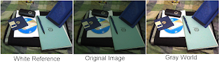
For this activity, we are to perform 2 different white balancing techniques, called the reference white algorithm and the gray world algorithm. In the reference white algorithm, a reference white object's pixel values are to be used to normalize the red, green and blue channels of the whole image. On the other hand, gray world algorithm uses the mean of each of the RGB channel values as the normalization factor.
We used two sets of objects for this activity. One set is a set of objects with different colors and another set is a set of objects with the same colors. For my second set I used a blue set of objects. The images were taken under a fluorescent lamp using the "tungsten", "daylight" and "cloudy" white balancing settings of a Canon Powershot A460 digital camera.
The following are the results for object with different colors:
 TUNGSTEN
 CLOUDY
 DAYLIGHT
For all the images, Reference white algorithm seems to work better since the gray world algorithm requires a certain constant to be multiplied to reduce the brightness of the resulting image. For this part the constant used to limit the brightness is 0.75.
The following are the results for different blue objects under different white balancing conditions.
 CLOUDY
 DAYLIGHT
 TUNGSTEN
For images with the same color, the reference white algorithm clearly performs better. The results of the gray world algorithm produced images with slightly redder image. A possible reason is because an average of an ensemble of colors may become white but an ensemble of objects having similar colors is not necessarily white. Hence, the white reference algorithm is expected to perform better.
Scilab Code:
I = imread("IMG_0921_cloudy.jpg");
//start of reference white algorithm
imshow(I);
pos = locate(1);
Rw = I(pos(1),pos(2),1);
Gw = I(pos(1),pos(2),2);
Bw = I(pos(1),pos(2),3);
//Start of gray world algorithm
//Rw = mean(I(:,:,1));
//Gw = mean(I(:,:,2));
//Bw = mean(I(:,:,3));
I(:,:,1) = I(:,:,1)/Rw;
I(:,:,2) = I(:,:,2)/Gw;
I(:,:,3) = I(:,:,3)/Bw;
//I = I*0.5;
I(I>1) = 1;
imwrite(I,"enhanced_cloudy.jpg");
----------------------------------------------
10/10 for this activity since I was able to finish the activity quickly and correctly.
Collaborator: Eduardo David
Wednesday, August 6, 2008
Activity 13: Photometric Stereo
In this activity we are to reconstruct an image using different images taken from the same point with different point source locations. The following are the images used with their corresponding point source positions

Using the following formula, we were able to obtain a 3d plot for the original image


loadmatfile("Photos.mat");
scf(0);imshow(I1,[]);
scf(1);imshow(I2,[]);
scf(2);imshow(I3,[]);
scf(3);imshow(I4,[]);
V1 = [0.085832, 0.17365, 0.98106];
V2 = [0.085832, -0.17365, 0.98106];
V3 = [0.17365, 0, 0.98481];
V4 = [0.16318, -0.34202, 0.92542];
I(1,:) = I1(:)';
I(2,:) = I2(:)';
I(3,:) = I3(:)';
I(4,:) = I4(:)';
//I = cat(1,I1(:)',I2(:)',I3(:)',I4(:)');
V = cat(1,V1,V2,V3,V4);
g = inv(V'*V)*V'*I;
N = size(g);
for i = 1:N(2)
gMag(i) = sqrt(g(1,i)**2+g(2,i)**2+g(3,i)**2+0.0000000000001);
end
nh(1,:) = (g(1,:)./gMag');
nh(2,:) = (g(2,:)./gMag');
nh(3,:) = (g(3,:)./gMag')+0.0000000000001;
fx = -nh(1,:)./nh(3,:);
fx = matrix(fx,[128,128])
fy = -nh(2,:)./nh(3,:);
fy = matrix(fy,[128,128]);
f = cumsum(fx,2)+cumsum(fy,1);
plot3d(1:128,1:128,f);
I will grade myself 10 for this activity since I was able to meet the objectives.
Collaborator: Eduardo David
Wednesday, July 30, 2008
Activity 11: Camera Calibration
In this activity, we are to obtain transformation of the camera coordinates with real world coordinates using a checkerboard pattern shown below as a calibration object
 I assigned the bottom center of the image as my origin and the left part as the "x" axis and the right part as the "y" and the vertical direction as the "z". To calibrate the camera, first, we assigned 25 corner points chosen at random in the image (marked with yellow squares). The location of the points are obtained using the "locate" function of scilab.
To solve for the camera parameters, we use the following matrix:
 Where xo, yo and zo correspond to real world coordinates and yi and zi correspond to image coordinates. aij correspond to the camera parameters.
The camera parameter matrix can be solved using:
 Where Q is the matrix containing the real world coordinates and d is the matrix containing the image coordinates.
The camera parameters obtained are as follows:
To confirm if this camera parameters are correct, we use it to predict the locations of the selected points in the image from the real world coordinates. The following equation is applied:


Using the above equations I obtained the following results:
The 1st pair of data correspond to the actual image coordinates, 2nd pair correspond to the coordinates solved using the above equation and the 3rd pair corresponds to their difference.


 The average value of the difference is 0.359 with standard deviation of 0.318. This translates to an error of roughly 1%.
The scilab code I used is given below:
---------------------------------------------------------------------------------
I = imread("C:\Users\RAFAEL JACULBIA\Documents\subjects\186\activity11\marked.bmp");
I = im2gray(I);
//imshow(I,[]);
//d = [];
//d = locate(25,flag=1);
image = [7 4 0 0 6 1 0 4 0 7 1 0 2 5 0 0 0 7 2 0 4 0 7 1 0;
0 0 4 0 0 0 4 0 5 0 0 2 0 0 0 3 7 0 0 2 0 4 0 0 6;
11 11 11 10 9 9 9 8 8 7 7 7 6 5 5 5 5 3 3 3 2 2 1 1 1];
//image = image*72;
Q = [];
yi = [];
zi = [];
for i = 1:25
x = image(1,i);
y = image(2,i);
z = image(3,i);
yi = d(1,i);
zi = d(2,i);
Qi = [x y z 1 0 0 0 0 -(yi*x) -(yi*y) -(yi*z); 0 0 0 0 x y z 1 -(zi*x) -(zi*y) -(zi*z)];
Q = cat(1, Q, Qi);
end
d2 = [];
d2 = matrix(d, 50,1);
a = inv(Q'*Q)*Q'*d2;
for j = 1:25
yi2(j) = ((a(1)*image(1,j))+(a(2)*image(2,j))+(a(3)*image(3,j))+a(4))/((a(9)*image(1,j))+(a(10)*image(2,j))+(a(11)*image(3,j))+1);
zi2(j) = ((a(5)*image(1,j))+(a(6)*image(2,j))+(a(7)*image(3,j))+a(8))/((a(9)*image(1,j))+(a(10)*image(2,j))+(a(11)*image(3,j))+1);
end
for k = 1:25
yi(k) = d(1,k);
zi(k) = d(2,k);
end
tryx = 0;
tryy = 6;
tryz = 1;
yiTry = ((a(1)*tryx)+(a(2)*tryy)+(a(3)*tryz)+a(4))/((a(9)*tryx)+(a(10)*tryy)+(a(11)*tryz)+1)
ziTry = ((a(5)*tryx)+(a(6)*tryy)+(a(7)*tryz)+a(8))/((a(9)*tryx)+(a(10)*tryy)+(a(11)*tryz)+1)
-------------------------------------------------------------------------------------------
For this activity I will give myself a grade of 10 because I was able to obtain quite accurate results.
Thanks to Eduardo David for teaching me how to resize a matrix in scilab


 I assigned the bottom center of the image as my origin and the left part as the "x" axis and the right part as the "y" and the vertical direction as the "z". To calibrate the camera, first, we assigned 25 corner points chosen at random in the image (marked with yellow squares). The location of the points are obtained using the "locate" function of scilab.
To solve for the camera parameters, we use the following matrix:
 Where xo, yo and zo correspond to real world coordinates and yi and zi correspond to image coordinates. aij correspond to the camera parameters.
The camera parameter matrix can be solved using:
 Where Q is the matrix containing the real world coordinates and d is the matrix containing the image coordinates.
The camera parameters obtained are as follows:
| -19.19404 |
| 9.7237133 |
| -0.5773294 |
| 167.80985 |
| -2.5034951 |
| -3.831655 |
| 20.477795 |
| 32.311712 |
| -0.0067168 |
| -0.0120008 |
| -0.0025509 |
To confirm if this camera parameters are correct, we use it to predict the locations of the selected points in the image from the real world coordinates. The following equation is applied:

Using the above equations I obtained the following results:
The 1st pair of data correspond to the actual image coordinates, 2nd pair correspond to the coordinates solved using the above equation and the 3rd pair corresponds to their difference.
| Image Coordinates | Solved Coordinates | difference | |||
| yi | zi | yi | zi | yi | zi |
| 29.096045 | 259.60452 | 29.300782 | 259.52771 | 0.204737 | 0.07681 |
| 89.548023 | 262.42938 | 89.604812 | 261.94118 | 0.056789 | 0.4882 |
| 216.66667 | 261.86441 | 216.84828 | 262.18338 | 0.18161 | 0.31897 |
| 166.38418 | 243.22034 | 166.27818 | 243.29594 | 0.106 | 0.0756 |
| 50 | 214.97175 | 50.653965 | 215.20451 | 0.653965 | 0.23276 |
| 147.74011 | 220.62147 | 147.806 | 220.65636 | 0.06589 | 0.03489 |
| 217.23164 | 216.66667 | 216.9003 | 216.65975 | 0.33134 | 0.00692 |
| 91.242938 | 194.63277 | 90.702993 | 195.35542 | 0.539945 | 0.72265 |
| 229.66102 | 192.37288 | 230.33101 | 192.45105 | 0.66999 | 0.07817 |
| 31.920904 | 169.20904 | 31.45059 | 169.10213 | 0.470314 | 0.10691 |
| 147.74011 | 176.55367 | 148.21666 | 177.51489 | 0.47655 | 0.96122 |
| 191.24294 | 175.9887 | 191.22007 | 175.33202 | 0.02287 | 0.65668 |
| 129.66102 | 155.08475 | 129.68482 | 154.61499 | 0.0238 | 0.46976 |
| 73.163842 | 127.9661 | 72.303439 | 128.12011 | 0.860403 | 0.15401 |
| 167.51412 | 137.00565 | 167.05391 | 136.44094 | 0.46021 | 0.56471 |
| 204.80226 | 130.22599 | 204.04286 | 129.52077 | 0.7594 | 0.70522 |
| 258.47458 | 119.49153 | 257.94833 | 119.43573 | 0.52625 | 0.0558 |
| 33.050847 | 81.073446 | 33.55399 | 80.628618 | 0.503143 | 0.444828 |
| 129.66102 | 90.677966 | 130.44029 | 90.649574 | 0.77927 | 0.028392 |
| 191.24294 | 88.983051 | 191.58995 | 88.895726 | 0.34701 | 0.087325 |
| 92.937853 | 65.254237 | 92.847265 | 65.342247 | 0.090588 | 0.08801 |
| 217.23164 | 60.169492 | 217.07798 | 61.190191 | 0.15366 | 1.020699 |
| 34.745763 | 37.00565 | 34.588753 | 37.10424 | 0.15701 | 0.09859 |
| 149.43503 | 50.564972 | 149.42329 | 50.756407 | 0.01174 | 0.191435 |
| 243.22034 | 32.485876 | 243.74758 | 32.200294 | 0.52724 | 0.285582 |
The average value of the difference is 0.359 with standard deviation of 0.318. This translates to an error of roughly 1%. The scilab code I used is given below:
---------------------------------------------------------------------------------
I = imread("C:\Users\RAFAEL JACULBIA\Documents\subjects\186\activity11\marked.bmp");
I = im2gray(I);
//imshow(I,[]);
//d = [];
//d = locate(25,flag=1);
image = [7 4 0 0 6 1 0 4 0 7 1 0 2 5 0 0 0 7 2 0 4 0 7 1 0;
0 0 4 0 0 0 4 0 5 0 0 2 0 0 0 3 7 0 0 2 0 4 0 0 6;
11 11 11 10 9 9 9 8 8 7 7 7 6 5 5 5 5 3 3 3 2 2 1 1 1];
//image = image*72;
Q = [];
yi = [];
zi = [];
for i = 1:25
x = image(1,i);
y = image(2,i);
z = image(3,i);
yi = d(1,i);
zi = d(2,i);
Qi = [x y z 1 0 0 0 0 -(yi*x) -(yi*y) -(yi*z); 0 0 0 0 x y z 1 -(zi*x) -(zi*y) -(zi*z)];
Q = cat(1, Q, Qi);
end
d2 = [];
d2 = matrix(d, 50,1);
a = inv(Q'*Q)*Q'*d2;
for j = 1:25
yi2(j) = ((a(1)*image(1,j))+(a(2)*image(2,j))+(a(3)*image(3,j))+a(4))/((a(9)*image(1,j))+(a(10)*image(2,j))+(a(11)*image(3,j))+1);
zi2(j) = ((a(5)*image(1,j))+(a(6)*image(2,j))+(a(7)*image(3,j))+a(8))/((a(9)*image(1,j))+(a(10)*image(2,j))+(a(11)*image(3,j))+1);
end
for k = 1:25
yi(k) = d(1,k);
zi(k) = d(2,k);
end
tryx = 0;
tryy = 6;
tryz = 1;
yiTry = ((a(1)*tryx)+(a(2)*tryy)+(a(3)*tryz)+a(4))/((a(9)*tryx)+(a(10)*tryy)+(a(11)*tryz)+1)
ziTry = ((a(5)*tryx)+(a(6)*tryy)+(a(7)*tryz)+a(8))/((a(9)*tryx)+(a(10)*tryy)+(a(11)*tryz)+1)
-------------------------------------------------------------------------------------------
For this activity I will give myself a grade of 10 because I was able to obtain quite accurate results.
Thanks to Eduardo David for teaching me how to resize a matrix in scilab
Tuesday, July 22, 2008
Activity 10: Preprocessing Handwritten Text
For this activity, the goal is to extract text from an imaged documents with lines. The given document is as follows (image resized):

I cropped a small portion of the image for faster calculations. The cropped image and its FT is shown below:
 To remove the vertical and horizontal lines I applied the following filter and the image beside it is the resulting image, also included is the binarized version of the image:

It can be seen that the lines are not actually removed totally, specially at the edges. In the image we can see that only the 1st line column can be read and last column is totally unreadable. To further enhance the image I performed opening and closing to isolate some of the letters using a 2x1 structuring element. And to make the letters 1 pixel thick, I performed erosion using the same structuring element. Afterwards, I labeled the text using bwlabel, the following image is the result:

As expected only some of the text are readable, almost all of the the numbers on the 1st column and the fractions on the second column are readable, but the third to fifth columns are pretty much unreadable.
The whole scilab code I used is shown below, it is a "mixture" of my older codes so it may look familiar. =)
------------------------------------------------------------------------------------
I = imread("C:\Users\RAFAEL JACULBIA\Documents\subjects\186\activity10\last\small.bmp");
I2 = im2gray(I);
C = imread("C:\Users\RAFAEL JACULBIA\Documents\subjects\186\activity10\last\cross.bmp");
C = im2gray(C);
Cshift = fftshift(C);
ftI = fft2(I2);
conv = Cshift.*ftI;
iconv = fft2(conv);
iconv = abs(fft2(fft2(iconv)));
scf(0);imshow(I2,[]);
scf(1);imshow(iconv,[]);
imwrite(iconv/max(iconv), "C:\Users\RAFAEL JACULBIA\Documents\subjects\186\activity10\last\noLines.bmp");
imwrite(abs(fft2(fft2(iconv)))/max(abs(fft2(fft2(iconv)))), "C:\Users\RAFAEL JACULBIA\Documents\subjects\186\activity10\last\res.bmp");
bw = im2bw(iconv,0.5);
imwrite(bw, "C:\Users\RAFAEL JACULBIA\Documents\subjects\186\activity10\last\bw.bmp");
scf(3);imshow(bw,[]);
bw = abs(bw-1);
se = [1,1];
OC = erode(dilate(dilate(erode(bw,se),se),se),se);
OC = erode(OC,se);
L = bwlabel(OC);
scf(4);imshow(L,[]);
imwrite(L/max(L), "C:\Users\RAFAEL JACULBIA\Documents\subjects\186\activity10\last\labeled.bmp");
------------------------------------------------------------------------------------------
For this activity, I will give myself a grade of 9/10 since I believe I was not able to accomplish the tasks perfectly. And for the first time I performed the activity without the help of others.

I cropped a small portion of the image for faster calculations. The cropped image and its FT is shown below:
 To remove the vertical and horizontal lines I applied the following filter and the image beside it is the resulting image, also included is the binarized version of the image:
It can be seen that the lines are not actually removed totally, specially at the edges. In the image we can see that only the 1st line column can be read and last column is totally unreadable. To further enhance the image I performed opening and closing to isolate some of the letters using a 2x1 structuring element. And to make the letters 1 pixel thick, I performed erosion using the same structuring element. Afterwards, I labeled the text using bwlabel, the following image is the result:

As expected only some of the text are readable, almost all of the the numbers on the 1st column and the fractions on the second column are readable, but the third to fifth columns are pretty much unreadable.
The whole scilab code I used is shown below, it is a "mixture" of my older codes so it may look familiar. =)
------------------------------------------------------------------------------------
I = imread("C:\Users\RAFAEL JACULBIA\Documents\subjects\186\activity10\last\small.bmp");
I2 = im2gray(I);
C = imread("C:\Users\RAFAEL JACULBIA\Documents\subjects\186\activity10\last\cross.bmp");
C = im2gray(C);
Cshift = fftshift(C);
ftI = fft2(I2);
conv = Cshift.*ftI;
iconv = fft2(conv);
iconv = abs(fft2(fft2(iconv)));
scf(0);imshow(I2,[]);
scf(1);imshow(iconv,[]);
imwrite(iconv/max(iconv), "C:\Users\RAFAEL JACULBIA\Documents\subjects\186\activity10\last\noLines.bmp");
imwrite(abs(fft2(fft2(iconv)))/max(abs(fft2(fft2(iconv)))), "C:\Users\RAFAEL JACULBIA\Documents\subjects\186\activity10\last\res.bmp");
bw = im2bw(iconv,0.5);
imwrite(bw, "C:\Users\RAFAEL JACULBIA\Documents\subjects\186\activity10\last\bw.bmp");
scf(3);imshow(bw,[]);
bw = abs(bw-1);
se = [1,1];
OC = erode(dilate(dilate(erode(bw,se),se),se),se);
OC = erode(OC,se);
L = bwlabel(OC);
scf(4);imshow(L,[]);
imwrite(L/max(L), "C:\Users\RAFAEL JACULBIA\Documents\subjects\186\activity10\last\labeled.bmp");
------------------------------------------------------------------------------------------
For this activity, I will give myself a grade of 9/10 since I believe I was not able to accomplish the tasks perfectly. And for the first time I performed the activity without the help of others.
Sunday, July 20, 2008
Activity 9: Binary Operations
In this activity, we are to measure the individual areas of a number of punched paper. It is assumed that the areas of the punched paper are uniform. The image I used is Circles001.jpg shown below:
 For faster calculations, I subdivided the images into 10, 256x256pixel images. A typical subdivision is shown below:
 Closing and Opening operators are necessary to be able to separate nearly touching circles and to clean the edges of broken circles. In general opening and closing operators are "mixtures" of dilation and erosion operator from the previous activity. Opening operations is achieved by dilating an eroded image. That is we are to perform erosion on an image then perform dilation on the resulting image. On the other hand, Closing is achieved in the opposite manner, in this case, performing erosion on a dilated image. Since erosion and dilation requires binary images, I binarized the subimages using 0.8 as a threshold. The code I used for the whole process is given below:
----------------------------------------------------------------------
I = imread("C:\Users\RAFAEL JACULBIA\Documents\subjects\186\activity9\C1_10.bmp");
se = imread("C:\Users\RAFAEL JACULBIA\Documents\subjects\186\activity9\disk.bmp");
bw = im2bw(I,0.8);
OC = erode(dilate(dilate(erode(bw,se),se),se),se);
L = bwlabel(OC);
imshow(L,[]);
imwrite(L/max(L), "C:\Users\RAFAEL JACULBIA\Documents\subjects\186\activity9\C1_10_labeled.bmp");
//imwrite(CO/max(CO), "C:\Users\RAFAEL JACULBIA\Documents\subjects\186\activity9\c2\C2_01_labeled2.bmp");
//imwrite(OC/max(OC), "C:\Users\RAFAEL JACULBIA\Documents\subjects\186\activity9\c2\C2_01_labeled3.bmp");
//imwrite(clos/max(clos), "C:\Users\RAFAEL JACULBIA\Documents\subjects\186\activity9\c2\C2_01_labeled4.bmp");
scircle = [];
for i=1:max(L)
circle = size(find(L==i));
scircle(i) = circle(2);
end
scircle
----------------------------------------------------------------------------
The structuring element I used was a 5x5 pixel "circle" which actually looks more like a cross than a circle drawn using GIMP. I performed opening and then closing operations on the images. In the code I displayed the resulting image with different circles "labeled" a typical image is shown below:
 The areas of all subimages were tallied and a histogram of the values were obtained:

I selected only areas between 300 and 800, since I believe areas out of this range are either circles grouped together or small pixels which are the result of dividing the images or is an artifact of binarizing the images. The value with largest occurence was found at 547 pixels. To confirm if this value is correct, I measured the diameter of one circle and found it to be 26 pixels corresponding to an area of 530 pixels, hence the obtained areas was near the calculated values. Another method I used to confirm the area is isolating a single circle, binarizing it and counting the number of pixels. Using this method I was able to obtain an area equal to 536 pixels which is still near the calculated value.
I also tried entering the whole image into scilab. It is interesting to note that limiting the values for area is not neccessary if we performed the operation on the whole image. I was able to obtain an area of 557.8 which is near the value obtained if I subdivided the images. The histogram is given below:

For this activity I will give myself a grade of 10 since I believe I have performed the activity correctly.
Eduardo David Helped me in this activity.
 For faster calculations, I subdivided the images into 10, 256x256pixel images. A typical subdivision is shown below:
 Closing and Opening operators are necessary to be able to separate nearly touching circles and to clean the edges of broken circles. In general opening and closing operators are "mixtures" of dilation and erosion operator from the previous activity. Opening operations is achieved by dilating an eroded image. That is we are to perform erosion on an image then perform dilation on the resulting image. On the other hand, Closing is achieved in the opposite manner, in this case, performing erosion on a dilated image. Since erosion and dilation requires binary images, I binarized the subimages using 0.8 as a threshold. The code I used for the whole process is given below:
----------------------------------------------------------------------
I = imread("C:\Users\RAFAEL JACULBIA\Documents\subjects\186\activity9\C1_10.bmp");
se = imread("C:\Users\RAFAEL JACULBIA\Documents\subjects\186\activity9\disk.bmp");
bw = im2bw(I,0.8);
OC = erode(dilate(dilate(erode(bw,se),se),se),se);
L = bwlabel(OC);
imshow(L,[]);
imwrite(L/max(L), "C:\Users\RAFAEL JACULBIA\Documents\subjects\186\activity9\C1_10_labeled.bmp");
//imwrite(CO/max(CO), "C:\Users\RAFAEL JACULBIA\Documents\subjects\186\activity9\c2\C2_01_labeled2.bmp");
//imwrite(OC/max(OC), "C:\Users\RAFAEL JACULBIA\Documents\subjects\186\activity9\c2\C2_01_labeled3.bmp");
//imwrite(clos/max(clos), "C:\Users\RAFAEL JACULBIA\Documents\subjects\186\activity9\c2\C2_01_labeled4.bmp");
scircle = [];
for i=1:max(L)
circle = size(find(L==i));
scircle(i) = circle(2);
end
scircle
----------------------------------------------------------------------------
The structuring element I used was a 5x5 pixel "circle" which actually looks more like a cross than a circle drawn using GIMP. I performed opening and then closing operations on the images. In the code I displayed the resulting image with different circles "labeled" a typical image is shown below:
 The areas of all subimages were tallied and a histogram of the values were obtained:
I selected only areas between 300 and 800, since I believe areas out of this range are either circles grouped together or small pixels which are the result of dividing the images or is an artifact of binarizing the images. The value with largest occurence was found at 547 pixels. To confirm if this value is correct, I measured the diameter of one circle and found it to be 26 pixels corresponding to an area of 530 pixels, hence the obtained areas was near the calculated values. Another method I used to confirm the area is isolating a single circle, binarizing it and counting the number of pixels. Using this method I was able to obtain an area equal to 536 pixels which is still near the calculated value.
I also tried entering the whole image into scilab. It is interesting to note that limiting the values for area is not neccessary if we performed the operation on the whole image. I was able to obtain an area of 557.8 which is near the value obtained if I subdivided the images. The histogram is given below:

For this activity I will give myself a grade of 10 since I believe I have performed the activity correctly.
Eduardo David Helped me in this activity.
Tuesday, July 15, 2008
Activity 8: Morphological Operations
For this activity, we are to predict and simulate the effects of the morphological operations dilation and erosion on some polygons. We are to perform dilation and erosion on a binary image of a square (50×50) , a triangle (base = 50 , height= 30), a circle (radius 25), a hollow square (60×60, edges are 4 pixels thick), and a plus sign (8 pixels thick and 50 pixels long for each line).
I used a 4x4, 2x4, 4x2 and a cross, 5 pixels long, one pixel thick as structuring elements drawn using GIMP.
The following are my predictions:


To confirm the predictions I used the following code:
------------------------------------------------------------
Obj = imread("C:\Users\RAFAEL JACULBIA\Documents\subjects\186\activity8\triangle.bmp");
Obj = im2bw(Obj,1);
se1 = imread("C:\Users\RAFAEL JACULBIA\Documents\subjects\186\activity8\4x4.bmp");
se2 = imread("C:\Users\RAFAEL JACULBIA\Documents\subjects\186\activity8\2x4.bmp");
se3 = imread("C:\Users\RAFAEL JACULBIA\Documents\subjects\186\activity8\4x2.bmp");
se4 = imread("C:\Users\RAFAEL JACULBIA\Documents\subjects\186\activity8\cross.bmp");
E1d = dilate(Obj,se1,[1,1]);
E2d = dilate(Obj,se2,[1,1]);
E3d = dilate(Obj,se3,[1,1]);
E4d = dilate(Obj,se4);
E1e = erode(Obj,se1,[1,1]);
E2e = erode(Obj,se2,[1,1]);
E3e = erode(Obj,se3,[1,1]);
E4e = erode(Obj,se4);
scf(0);imshow(E1d,[]);
//scf(1);imshow(E2,[]);
imwrite(E1d,"C:\Users\RAFAEL JACULBIA\Documents\subjects\186\activity8\triangle\4x4triangle_dilate.bmp");
imwrite(E2d,"C:\Users\RAFAEL JACULBIA\Documents\subjects\186\activity8\triangle\2x4triangle_dilate.bmp");
imwrite(E3d,"C:\Users\RAFAEL JACULBIA\Documents\subjects\186\activity8\triangle\4x2triangle_dilate.bmp");
imwrite(E4d,"C:\Users\RAFAEL JACULBIA\Documents\subjects\186\activity8\triangle\crosStriangle_dilate.bmp");
imwrite(E1e,"C:\Users\RAFAEL JACULBIA\Documents\subjects\186\activity8\triangle\4x4triangle_erode.bmp");
imwrite(E2e,"C:\Users\RAFAEL JACULBIA\Documents\subjects\186\activity8\triangle\2x4triangle_erode.bmp");
imwrite(E3e,"C:\Users\RAFAEL JACULBIA\Documents\subjects\186\activity8\triangle\4x2triangle_erode.bmp");
imwrite(E4e,"C:\Users\RAFAEL JACULBIA\Documents\subjects\186\activity8\triangle\crosStriangle_erode.bmp");
--------------------------------------------------
The following shows the results obtained for a square object:

The following are the results for the triangle
The Following are the results for the circle
The following are the results for the hollow square

The following are the results for the plus sign.
In general most of my predictions are correct specially for the cross and the square, but for the triangle and hollow square I believe I did not predict the result exactly. For the circle I was only correct on the size but on the general shape I believe I was not correct, (e.g. flatten edges of the circle).
For this I will give myself a great of 8/10 since I was not able to predict all of the results perfectly and at first I really did not understand the effects on a hollow square.
Many Thanks to the following people who helped me a lot in this activity.
Eduardo David
Elizabeth Ann Prieto
I used a 4x4, 2x4, 4x2 and a cross, 5 pixels long, one pixel thick as structuring elements drawn using GIMP.
The following are my predictions:


To confirm the predictions I used the following code:
------------------------------------------------------------
Obj = imread("C:\Users\RAFAEL JACULBIA\Documents\subjects\186\activity8\triangle.bmp");
Obj = im2bw(Obj,1);
se1 = imread("C:\Users\RAFAEL JACULBIA\Documents\subjects\186\activity8\4x4.bmp");
se2 = imread("C:\Users\RAFAEL JACULBIA\Documents\subjects\186\activity8\2x4.bmp");
se3 = imread("C:\Users\RAFAEL JACULBIA\Documents\subjects\186\activity8\4x2.bmp");
se4 = imread("C:\Users\RAFAEL JACULBIA\Documents\subjects\186\activity8\cross.bmp");
E1d = dilate(Obj,se1,[1,1]);
E2d = dilate(Obj,se2,[1,1]);
E3d = dilate(Obj,se3,[1,1]);
E4d = dilate(Obj,se4);
E1e = erode(Obj,se1,[1,1]);
E2e = erode(Obj,se2,[1,1]);
E3e = erode(Obj,se3,[1,1]);
E4e = erode(Obj,se4);
scf(0);imshow(E1d,[]);
//scf(1);imshow(E2,[]);
imwrite(E1d,"C:\Users\RAFAEL JACULBIA\Documents\subjects\186\activity8\triangle\4x4triangle_dilate.bmp");
imwrite(E2d,"C:\Users\RAFAEL JACULBIA\Documents\subjects\186\activity8\triangle\2x4triangle_dilate.bmp");
imwrite(E3d,"C:\Users\RAFAEL JACULBIA\Documents\subjects\186\activity8\triangle\4x2triangle_dilate.bmp");
imwrite(E4d,"C:\Users\RAFAEL JACULBIA\Documents\subjects\186\activity8\triangle\crosStriangle_dilate.bmp");
imwrite(E1e,"C:\Users\RAFAEL JACULBIA\Documents\subjects\186\activity8\triangle\4x4triangle_erode.bmp");
imwrite(E2e,"C:\Users\RAFAEL JACULBIA\Documents\subjects\186\activity8\triangle\2x4triangle_erode.bmp");
imwrite(E3e,"C:\Users\RAFAEL JACULBIA\Documents\subjects\186\activity8\triangle\4x2triangle_erode.bmp");
imwrite(E4e,"C:\Users\RAFAEL JACULBIA\Documents\subjects\186\activity8\triangle\crosStriangle_erode.bmp");
--------------------------------------------------
The following shows the results obtained for a square object:

The following are the results for the triangle

The Following are the results for the circle

The following are the results for the hollow square

The following are the results for the plus sign.

In general most of my predictions are correct specially for the cross and the square, but for the triangle and hollow square I believe I did not predict the result exactly. For the circle I was only correct on the size but on the general shape I believe I was not correct, (e.g. flatten edges of the circle).
For this I will give myself a great of 8/10 since I was not able to predict all of the results perfectly and at first I really did not understand the effects on a hollow square.
Many Thanks to the following people who helped me a lot in this activity.
Eduardo David
Elizabeth Ann Prieto
Subscribe to:
Comments (Atom)