Activity 11: Camera Calibration

In this activity, we are to obtain transformation of the camera coordinates with real world coordinates using a checkerboard pattern shown below as a calibration object
I assigned the bottom center of the image as my origin and the left part as the "x" axis and the right part as the "y" and the vertical direction as the "z". To calibrate the camera, first, we assigned 25 corner points chosen at random in the image (marked with yellow squares). The location of the points are obtained using the "locate" function of scilab.
To solve for the camera parameters, we use the following matrix:
Where xo, yo and zo correspond to real world coordinates and yi and zi correspond to image coordinates. aij correspond to the camera parameters.
The camera parameter matrix can be solved using:
Where Q is the matrix containing the real world coordinates and d is the matrix containing the image coordinates.
The camera parameters obtained are as follows:

-19.19404
9.7237133
-0.5773294
167.80985
-2.5034951
-3.831655
20.477795
32.311712
-0.0067168
-0.0120008
-0.0025509

To confirm if this camera parameters are correct, we use it to predict the locations of the selected points in the image from the real world coordinates. The following equation is applied:

Using the above equations I obtained the following results:
The 1st pair of data correspond to the actual image coordinates, 2nd pair correspond to the coordinates solved using the above equation and the 3rd pair corresponds to their difference.

Image Coordinates		Solved Coordinates		difference
yi	zi	yi	zi	yi	zi
29.096045	259.60452	29.300782	259.52771	0.204737	0.07681
89.548023	262.42938	89.604812	261.94118	0.056789	0.4882
216.66667	261.86441	216.84828	262.18338	0.18161	0.31897
166.38418	243.22034	166.27818	243.29594	0.106	0.0756
50	214.97175	50.653965	215.20451	0.653965	0.23276
147.74011	220.62147	147.806	220.65636	0.06589	0.03489
217.23164	216.66667	216.9003	216.65975	0.33134	0.00692
91.242938	194.63277	90.702993	195.35542	0.539945	0.72265
229.66102	192.37288	230.33101	192.45105	0.66999	0.07817
31.920904	169.20904	31.45059	169.10213	0.470314	0.10691
147.74011	176.55367	148.21666	177.51489	0.47655	0.96122
191.24294	175.9887	191.22007	175.33202	0.02287	0.65668
129.66102	155.08475	129.68482	154.61499	0.0238	0.46976
73.163842	127.9661	72.303439	128.12011	0.860403	0.15401
167.51412	137.00565	167.05391	136.44094	0.46021	0.56471
204.80226	130.22599	204.04286	129.52077	0.7594	0.70522
258.47458	119.49153	257.94833	119.43573	0.52625	0.0558
33.050847	81.073446	33.55399	80.628618	0.503143	0.444828
129.66102	90.677966	130.44029	90.649574	0.77927	0.028392
191.24294	88.983051	191.58995	88.895726	0.34701	0.087325
92.937853	65.254237	92.847265	65.342247	0.090588	0.08801
217.23164	60.169492	217.07798	61.190191	0.15366	1.020699
34.745763	37.00565	34.588753	37.10424	0.15701	0.09859
149.43503	50.564972	149.42329	50.756407	0.01174	0.191435
243.22034	32.485876	243.74758	32.200294	0.52724	0.285582

The average value of the difference is 0.359 with standard deviation of 0.318. This translates to an error of roughly 1%.

The scilab code I used is given below:
---------------------------------------------------------------------------------
I = imread("C:\Users\RAFAEL JACULBIA\Documents\subjects\186\activity11\marked.bmp");
I = im2gray(I);
//imshow(I,[]);
//d = [];
//d = locate(25,flag=1);

image = [7 4 0 0 6 1 0 4 0 7 1 0 2 5 0 0 0 7 2 0 4 0 7 1 0;
0 0 4 0 0 0 4 0 5 0 0 2 0 0 0 3 7 0 0 2 0 4 0 0 6;
11 11 11 10 9 9 9 8 8 7 7 7 6 5 5 5 5 3 3 3 2 2 1 1 1];


//image = image*72;

Q = [];
yi = [];
zi = [];
for i = 1:25
x = image(1,i);
y = image(2,i);
z = image(3,i);
yi = d(1,i);
zi = d(2,i);
Qi = [x y z 1 0 0 0 0 -(yi*x) -(yi*y) -(yi*z); 0 0 0 0 x y z 1 -(zi*x) -(zi*y) -(zi*z)];
Q = cat(1, Q, Qi);
end
d2 = [];
d2 = matrix(d, 50,1);
a = inv(Q'*Q)*Q'*d2;

for j = 1:25
yi2(j) = ((a(1)*image(1,j))+(a(2)*image(2,j))+(a(3)*image(3,j))+a(4))/((a(9)*image(1,j))+(a(10)*image(2,j))+(a(11)*image(3,j))+1);
zi2(j) = ((a(5)*image(1,j))+(a(6)*image(2,j))+(a(7)*image(3,j))+a(8))/((a(9)*image(1,j))+(a(10)*image(2,j))+(a(11)*image(3,j))+1);
end

for k = 1:25
yi(k) = d(1,k);
zi(k) = d(2,k);
end

tryx = 0;
tryy = 6;
tryz = 1;

yiTry = ((a(1)*tryx)+(a(2)*tryy)+(a(3)*tryz)+a(4))/((a(9)*tryx)+(a(10)*tryy)+(a(11)*tryz)+1)
ziTry = ((a(5)*tryx)+(a(6)*tryy)+(a(7)*tryz)+a(8))/((a(9)*tryx)+(a(10)*tryy)+(a(11)*tryz)+1)
-------------------------------------------------------------------------------------------

For this activity I will give myself a grade of 10 because I was able to obtain quite accurate results.
Thanks to Eduardo David for teaching me how to resize a matrix in scilab

Activity 10: Preprocessing Handwritten Text

For this activity, the goal is to extract text from an imaged documents with lines. The given document is as follows (image resized):

I cropped a small portion of the image for faster calculations. The cropped image and its FT is shown below:
To remove the vertical and horizontal lines I applied the following filter and the image beside it is the resulting image, also included is the binarized version of the image:


It can be seen that the lines are not actually removed totally, specially at the edges. In the image we can see that only the 1st line column can be read and last column is totally unreadable. To further enhance the image I performed opening and closing to isolate some of the letters using a 2x1 structuring element. And to make the letters 1 pixel thick, I performed erosion using the same structuring element. Afterwards, I labeled the text using bwlabel, the following image is the result:


As expected only some of the text are readable, almost all of the the numbers on the 1st column and the fractions on the second column are readable, but the third to fifth columns are pretty much unreadable.
The whole scilab code I used is shown below, it is a "mixture" of my older codes so it may look familiar. =)
------------------------------------------------------------------------------------
I = imread("C:\Users\RAFAEL JACULBIA\Documents\subjects\186\activity10\last\small.bmp");
I2 = im2gray(I);
C = imread("C:\Users\RAFAEL JACULBIA\Documents\subjects\186\activity10\last\cross.bmp");
C = im2gray(C);
Cshift = fftshift(C);

ftI = fft2(I2);
conv = Cshift.*ftI;
iconv = fft2(conv);
iconv = abs(fft2(fft2(iconv)));
scf(0);imshow(I2,[]);
scf(1);imshow(iconv,[]);
imwrite(iconv/max(iconv), "C:\Users\RAFAEL JACULBIA\Documents\subjects\186\activity10\last\noLines.bmp");
imwrite(abs(fft2(fft2(iconv)))/max(abs(fft2(fft2(iconv)))), "C:\Users\RAFAEL JACULBIA\Documents\subjects\186\activity10\last\res.bmp");
bw = im2bw(iconv,0.5);
imwrite(bw, "C:\Users\RAFAEL JACULBIA\Documents\subjects\186\activity10\last\bw.bmp");
scf(3);imshow(bw,[]);

bw = abs(bw-1);
se = [1,1];



OC = erode(dilate(dilate(erode(bw,se),se),se),se);

OC = erode(OC,se);


L = bwlabel(OC);
scf(4);imshow(L,[]);

imwrite(L/max(L), "C:\Users\RAFAEL JACULBIA\Documents\subjects\186\activity10\last\labeled.bmp");
------------------------------------------------------------------------------------------

For this activity, I will give myself a grade of 9/10 since I believe I was not able to accomplish the tasks perfectly. And for the first time I performed the activity without the help of others.

Activity 9: Binary Operations

In this activity, we are to measure the individual areas of a number of punched paper. It is assumed that the areas of the punched paper are uniform. The image I used is Circles001.jpg shown below:
For faster calculations, I subdivided the images into 10, 256x256pixel images. A typical subdivision is shown below:
Closing and Opening operators are necessary to be able to separate nearly touching circles and to clean the edges of broken circles. In general opening and closing operators are "mixtures" of dilation and erosion operator from the previous activity. Opening operations is achieved by dilating an eroded image. That is we are to perform erosion on an image then perform dilation on the resulting image. On the other hand, Closing is achieved in the opposite manner, in this case, performing erosion on a dilated image. Since erosion and dilation requires binary images, I binarized the subimages using 0.8 as a threshold. The code I used for the whole process is given below:

----------------------------------------------------------------------
I = imread("C:\Users\RAFAEL JACULBIA\Documents\subjects\186\activity9\C1_10.bmp");
se = imread("C:\Users\RAFAEL JACULBIA\Documents\subjects\186\activity9\disk.bmp");
bw = im2bw(I,0.8);

OC = erode(dilate(dilate(erode(bw,se),se),se),se);
L = bwlabel(OC);
imshow(L,[]);

imwrite(L/max(L), "C:\Users\RAFAEL JACULBIA\Documents\subjects\186\activity9\C1_10_labeled.bmp");
//imwrite(CO/max(CO), "C:\Users\RAFAEL JACULBIA\Documents\subjects\186\activity9\c2\C2_01_labeled2.bmp");
//imwrite(OC/max(OC), "C:\Users\RAFAEL JACULBIA\Documents\subjects\186\activity9\c2\C2_01_labeled3.bmp");
//imwrite(clos/max(clos), "C:\Users\RAFAEL JACULBIA\Documents\subjects\186\activity9\c2\C2_01_labeled4.bmp");
scircle = [];
for i=1:max(L)
circle = size(find(L==i));
scircle(i) = circle(2);
end

scircle

----------------------------------------------------------------------------
The structuring element I used was a 5x5 pixel "circle" which actually looks more like a cross than a circle drawn using GIMP. I performed opening and then closing operations on the images. In the code I displayed the resulting image with different circles "labeled" a typical image is shown below:
The areas of all subimages were tallied and a histogram of the values were obtained:

I selected only areas between 300 and 800, since I believe areas out of this range are either circles grouped together or small pixels which are the result of dividing the images or is an artifact of binarizing the images. The value with largest occurence was found at 547 pixels. To confirm if this value is correct, I measured the diameter of one circle and found it to be 26 pixels corresponding to an area of 530 pixels, hence the obtained areas was near the calculated values. Another method I used to confirm the area is isolating a single circle, binarizing it and counting the number of pixels. Using this method I was able to obtain an area equal to 536 pixels which is still near the calculated value.

I also tried entering the whole image into scilab. It is interesting to note that limiting the values for area is not neccessary if we performed the operation on the whole image. I was able to obtain an area of 557.8 which is near the value obtained if I subdivided the images. The histogram is given below:




For this activity I will give myself a grade of 10 since I believe I have performed the activity correctly.

Eduardo David Helped me in this activity.

Activity 8: Morphological Operations

For this activity, we are to predict and simulate the effects of the morphological operations dilation and erosion on some polygons. We are to perform dilation and erosion on a binary image of a square (50×50) , a triangle (base = 50 , height= 30), a circle (radius 25), a hollow square (60×60, edges are 4 pixels thick), and a plus sign (8 pixels thick and 50 pixels long for each line).

I used a 4x4, 2x4, 4x2 and a cross, 5 pixels long, one pixel thick as structuring elements drawn using GIMP.

The following are my predictions:


To confirm the predictions I used the following code:

------------------------------------------------------------
Obj = imread("C:\Users\RAFAEL JACULBIA\Documents\subjects\186\activity8\triangle.bmp");
Obj = im2bw(Obj,1);

se1 = imread("C:\Users\RAFAEL JACULBIA\Documents\subjects\186\activity8\4x4.bmp");
se2 = imread("C:\Users\RAFAEL JACULBIA\Documents\subjects\186\activity8\2x4.bmp");
se3 = imread("C:\Users\RAFAEL JACULBIA\Documents\subjects\186\activity8\4x2.bmp");
se4 = imread("C:\Users\RAFAEL JACULBIA\Documents\subjects\186\activity8\cross.bmp");

E1d = dilate(Obj,se1,[1,1]);
E2d = dilate(Obj,se2,[1,1]);
E3d = dilate(Obj,se3,[1,1]);
E4d = dilate(Obj,se4);

E1e = erode(Obj,se1,[1,1]);
E2e = erode(Obj,se2,[1,1]);
E3e = erode(Obj,se3,[1,1]);
E4e = erode(Obj,se4);
scf(0);imshow(E1d,[]);
//scf(1);imshow(E2,[]);
imwrite(E1d,"C:\Users\RAFAEL JACULBIA\Documents\subjects\186\activity8\triangle\4x4triangle_dilate.bmp");
imwrite(E2d,"C:\Users\RAFAEL JACULBIA\Documents\subjects\186\activity8\triangle\2x4triangle_dilate.bmp");
imwrite(E3d,"C:\Users\RAFAEL JACULBIA\Documents\subjects\186\activity8\triangle\4x2triangle_dilate.bmp");
imwrite(E4d,"C:\Users\RAFAEL JACULBIA\Documents\subjects\186\activity8\triangle\crosStriangle_dilate.bmp");

imwrite(E1e,"C:\Users\RAFAEL JACULBIA\Documents\subjects\186\activity8\triangle\4x4triangle_erode.bmp");
imwrite(E2e,"C:\Users\RAFAEL JACULBIA\Documents\subjects\186\activity8\triangle\2x4triangle_erode.bmp");
imwrite(E3e,"C:\Users\RAFAEL JACULBIA\Documents\subjects\186\activity8\triangle\4x2triangle_erode.bmp");
imwrite(E4e,"C:\Users\RAFAEL JACULBIA\Documents\subjects\186\activity8\triangle\crosStriangle_erode.bmp");
--------------------------------------------------

The following shows the results obtained for a square object:



The following are the results for the triangle

The Following are the results for the circle
The following are the results for the hollow square


The following are the results for the plus sign.
In general most of my predictions are correct specially for the cross and the square, but for the triangle and hollow square I believe I did not predict the result exactly. For the circle I was only correct on the size but on the general shape I believe I was not correct, (e.g. flatten edges of the circle).

For this I will give myself a great of 8/10 since I was not able to predict all of the results perfectly and at first I really did not understand the effects on a hollow square.

Many Thanks to the following people who helped me a lot in this activity.
Eduardo David
Elizabeth Ann Prieto

Activity 7: Enhancement in the Frequency Domain

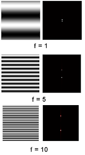
For the 1st part of this activity, we are to observe some properties of the fourier transform. First, we observed the effect of changing the frequency of the sinusoidal image. The following images shows the result for increasing frequency. Left images are the original 2D sinusoidal images while right ones are the fourier transform of the left images.

As expected, the FT of a sinusoidal image is a dot since from the previous activity the FT of a sinusoidal function is a delta function. As we increase the frequency, the spacing between the sinusoidal image increase, this has the effect of increasing the spacing of the delta function in fourier space. Hence, we observe the dots move apart as we increase frequency.

The next part of the activity is we tried to rotate the sinusoid by a factor of theta using the following formula:

The following results were obtained, again left images are the sinusoid images while the right are its corresponding fourier transform:
Rotating the sinusoid in has the effect of rotating its fourier transform in the clockwise direction.

Multiplication of two sinusoids produces a checkerboard image while its fourier transform are 4 dots along the edges:

The next objective is to enhance the appearance of the ridges of a fingerprint to enhance its appearance. The image I used is from the activity 7 manual, the original image, enhanced image the FT of the original image and the filter is shown below:

I chose to design the filter to mimic the fourier transform of the original image, I saved the FT of the original image then edited its contrast/brightness using GIMP. Convolving this filter with the original image would result in the removal of unwanted frequencies of the image. The resulted in an improved image of the fingerprint whose ridges are more clear than the original image. Also I noticed that discontinuities in the original image was removed after applying the filter.
The code that I used is given below:
-------------------------------------------------------------------------------------
I = imread("C:\Documents and Settings\semicon\Desktop\activity7\final\sample.bmp");
I2 = im2gray(I);
C = imread("C:\Documents and Settings\semicon\Desktop\activity7\final\ft.bmp");
C = im2gray(C);
Cshift = fftshift(C);

ftI = fft2(I2);
conv = Cshift.*ftI;
iconv = fft2(conv);
scf(0);imshow(I2,[]);
scf(1);imshow((abs(fft2(fft2(iconv)))),[]);
scf(2);imshow(log(fftshift(abs(ftI))), []);
xset("colormap",hotcolormap(256))
//imwrite(log(fftshift(abs(ftI)))/max(log(fftshift(abs(ftI)))), "C:\Documents and Settings\semicon\Desktop\activity7\final\ft.bmp");
//imwrite(abs(fft2(fft2(iconv)))/max(abs(fft2(fft2(iconv)))), "C:\Users\RAFAEL JACULBIA\Documents\subjects\186\activity7\final\hiRes.bmp");
----------------------------------------------------------------------------------

The next part of the activity aims to remove the vertical lines of an image of the moon's surface. For faster calculations, I resized the image to 270x203 pixels keeping the aspect ratio constant.
The original image, the improved image, the FT of the original image and the Filter used is shown below:


Saving the FT of the original image and adjusting it seems to be not working in this particular image so I tried to just mimic the FT instead of really editing it. It can be seen that the vertical lines of the original image is not visible anymore.


I will give myself a grade of 10 for this activity because the primary objectives were met. So far this activity seems to be the hardest for me, maybe because I am not really sure if I understand the method to be used.

Thanks to the following for helping me in this activity
Eduardo David
Elizabeth Ann Prieto
Jorge Michael Presto

Activity 6: Fourier Transform model of Image Formation

For this activity we performed fourier transform on images using the FFT2 function of scilab. For the first part we obtained the FFT of circles. The following image shows the FFT of a small circle.The leftmost image is the original image. The second to the left is the fourier transform (FT) of the original image, it can be seen that it is not consistent with the analytical FT of a circle. Shifting all the zero frequencies in the image produces the 3rd image, which is now consistent with the analytical FT of a circle which airy disks. The last image is the FT of the FT of the original image, it can be seen that the image returns to original which proves that FT is reversible. I also performed FT on a larger circle shown below.

It can be seen here that FFT becomes smaller as the image becomes larger, which is consistent with the theoretical expectations. FT was also performed in the letter A shown below:The important result for this part is that it confirms property 4 of the lecture. Which states that "The inverse FFT is just the same as the forward FFT with the image inverted"


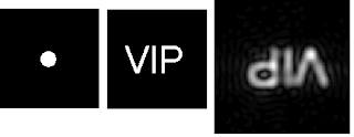
For part B of the activity we obtained the convolution of 2 images. One image serves as the "aperture" and the other serves as the "object." Taking the convolution of this two objects is similar to obtaining the "image" of the "object" using the "aperture" as a "lens." The following results are obtained for a small aperture
For a small aperture, fewer frequencies pass through. Hence we observe a bad reconstruction of the original image.


For a larger aperture, the results show that we are able to reconstruct a better image. However, we are still not able to obtain perfect reconstruction as seen in the image because the color of the image is not similar to the original.

For part C of the activity, we are to obtain the correlation of the a letter in a long sentence. We are to find the correlation of the letter "A" in the phrase "THE RAIN IN SPAIN STAYS MAINLY IN THE PLAIN." I used Arial font size 16, boldface for this part, the following is the code that I used:
-------------------------------------------------------
S = imread("C:\Documents and Settings\Semicon.POSITRON\Desktop\activity6\6C\sentence3.bmp");
A = imread("C:\Documents and Settings\Semicon.POSITRON\Desktop\activity6\6C\A3.bmp");
grayS = im2gray(S);
grayA = im2gray(A);
fftS = fft2(grayS);
fftA = fft2(grayA);
mul = fftA.*conj(fftS);
inve = fft2(mul);
scf(1);imshow(grayS);
scf(2);imshow(fftshift(abs((inve))),[]);
-------------------------------------------------------
I obtained the following result for the same sized A,

In this image we can see that the parts of the sentence where the letter "A" appears is somewhat highlighted. This is because high correlation is obtained for the parts where the letter A is present. I also tried to find the correlation of the same letter but with smaller font size, I obtained the following result:
Here we see that the phrase is more clear however, parts where the letter A appears is not highlighted.

For the last part of the activity, we performed edge detection on the word VIP using different patterns. I used the patterns suggested by Dr. Soriano, which are horizontal, vertical diagonal and spot.

The following code was used to implement the image detection using scilab:
-------------------------------------------------------------------
VIP = imread("C:\Documents and Settings\Semicon.POSITRON\Desktop\activity6\6d\T.bmp");
VIP = im2gray(VIP);
pattern1 = [-1 -1 -1;2 2 2; -1 -1 -1];
pattern2 = [-1 2 -1; -1 2 -1; -1 2 -1];
pattern3 = [2 -1 -1; -1 2 -1; -1 -1 2];
pattern4 = [-1 -1 -1; -1 8 -1; -1 -1 -1];

corre1 = imcorrcoef(VIP,pattern1);
corre2 = imcorrcoef(VIP,pattern2);
corre3 = imcorrcoef(VIP,pattern3);
corre4 = imcorrcoef(VIP,pattern4);

imwrite(corre1,"C:\Documents and Settings\Semicon.POSITRON\Desktop\activity6\6d\hori.bmp");
imwrite(corre2,"C:\Documents and Settings\Semicon.POSITRON\Desktop\activity6\6d\vert.bmp");
imwrite(corre3,"C:\Documents and Settings\Semicon.POSITRON\Desktop\activity6\6d\diag.bmp");
imwrite(corre4,"C:\Documents and Settings\Semicon.POSITRON\Desktop\activity6\6d\spot.bmp");

scf(0);imshow(corre1, []);
scf(1);imshow(corre2, []);
scf(2);imshow(corre3, []);
scf(3);imshow(corre4, []);

-----------------------------------------------------------------------
The following results were obtained for "VIP":

The arrangement is original, horizontal, vertical, diagonal and spot. For the horizontal, most of the vertical components are missing, for the vertical, the horizontal components are missing, for the diagonal some components from the vertical and horizontal are missing while for the spot most components are present. I tried using the algorithm in the letter "T" which highlighted the results further specially for the diagonal since, T almost has no diagonal components.

Obviously, components corresponding to the diagonal is almost absent and horizontal and vertical components for their corresponding filters are clear.

I will give myself a grade of 10 because I believe I was able to do all the required task and also I was able to completely explain the results.


Abraham Latimer Camba Helped me in this activity