For this activity, we classify the same set of objects as with activities 18 and 19 but using neural networks instead. A neural network will have three parts, the input layer, the hidden layer and the output layer. For classification purposes, the input layer contains the features and the output would contain the classes. As with activity 19 I used piatos and pillows as my 2 classes. The output may either be 0 (piatos) or 1 (pillows) depending on which class a sample belongs.
The code below follows the one written by Jeric. I used 4 input layer neurons, 8 hidden layer neurons and 1 output layer neuron. The following is the code I used, the training and test sets are the ones in activity 19.
-----------------------------------------------------------------------------------
chdir("C:\Users\RAFAEL JACULBIA\Documents\subjects\186\activity20");
N = [4,8,1];
train = fscanfMat("train.txt")';// Training Set
t = [0 0 0 0 1 1 1 1];
lp = [2.5,0];
W = ann_FF_init(N);
T = 500; //Training cyles
W = ann_FF_Std_online(train,t,N,W,lp,T);
test = fscanfMat("test2.txt")';
class = ann_FF_run(test,N,W)
round(class)
--------------------------------------------------------------------------
The following are the outputs of the program :
0.0723331 0.0343279 0.0358914 0.0102084 0.9948734 0.9865080 0.9895211 0.9913624
After rounding off, we see that the above outputs are 100% accurate.
I grade myself 10/10 for again getting a perfect classification. Thanks to jeric for the code and to ed for his help.
Thursday, October 9, 2008
Thursday, October 2, 2008
Activity 19: Probabilistic Classification
In this activity, we again classify different objects like what we did in activity 18. Only this time we perform linear discrimination analysis. It mainly assumes that our classes are separable by a linear combination of different features of the class. Class membership is attained for when a certain sample has minimum error of classification. A detailed discussion is given in Linear_Discrimant_Analysis_2.pdf by Dr. Sheila Marcos. The samples I used for this activity are piatos(class 1) and pillows (class 2). The features I used are: normalized area obtained via pixel counting, average value of the red component, ratio of the average value of the green component to the red component, and the ratio of the average value of the blue component to the red component. These parameters are obtained using the procedure described in my earlier post for activity 18. The first four samples are used as training set and the last four are used as the test set.
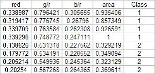
Using the above training set and the methods described in the provided pdf file, we can compute for the covariance matrix given below:
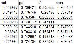
The test set is given below:
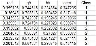
From this test set, the computed discrimant values are:
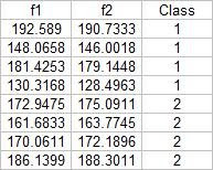 From these result it is obvious that I was able to obtain a 100% correct classification. I also tried this with a different sample combination (pillows vs squidballs) and I still got 100% correct classification. The following is the code I used:
-----------------------------------------------------------------------
chdir("C:\Users\RAFAEL JACULBIA\Documents\subjects\186\activity19");
x = [];
y = [];
x1 = [];
x2 = [];
u1 = [];
u2 = [];
x1o = [];
x2o = [];
c1 = [];
c2 = [];
C = [];
n = 8;
n1 = 4;
n2 = 4;
x = fscanfMat("x.txt");
y = fscanfMat("y.txt");
test = fscanfMat("test.txt");
x1 = x(1:n1,:);
x2 = x(n1+1:n,:);
u1 = mean(x1,'r');
u2 = mean(x2,'r');
u = mean(x,'r');
x1o(:,1) = x1(:,1) - u(:,1);
x1o(:,2) = x1(:,2) - u(:,2);
x1o(:,3) = x1(:,3) - u(:,3);
x1o(:,4) = x1(:,4) - u(:,4);
x2o(:,1) = x2(:,1) - u(:,1);
x2o(:,2) = x2(:,2) - u(:,2);
x2o(:,3) = x2(:,3) - u(:,3);
x2o(:,4) = x2(:,4) - u(:,4);
c1 = (x1o'*x1o)/n1;
c2 = (x2o'*x2o)/n2;
C = (n1/n)*c1 + (n2/n)*c2;
p = [n1/n;n2/n];
class = [];
for i = 1:size(test,1)
f1(i) = u1*inv(C)*test(i,:)'-0.5*u1*inv(C)*u1'+log(p(1));
f2(i) = u2*inv(C)*test(i,:)'-0.5*u2*inv(C)*u2'+log(p(2));
end
f1-f2
------------------------------------------------------------------------
I proudly grade myself 10/10 for getting it perfectly without the help of others. I also consider this activity one of the easiest because of the step by step method given in the provided file.

Using the above training set and the methods described in the provided pdf file, we can compute for the covariance matrix given below:
0.0062310 0.0087568 0.0012735 0.0226916
0.0087568 0.0129916 0.0019430 0.0329768
0.0012735 0.0019430 0.0005591 0.0042263
0.0226916 0.0329768 0.0042263 0.0876073
The test set is given below:

From this test set, the computed discrimant values are:
 From these result it is obvious that I was able to obtain a 100% correct classification. I also tried this with a different sample combination (pillows vs squidballs) and I still got 100% correct classification. The following is the code I used:
-----------------------------------------------------------------------
chdir("C:\Users\RAFAEL JACULBIA\Documents\subjects\186\activity19");
x = [];
y = [];
x1 = [];
x2 = [];
u1 = [];
u2 = [];
x1o = [];
x2o = [];
c1 = [];
c2 = [];
C = [];
n = 8;
n1 = 4;
n2 = 4;
x = fscanfMat("x.txt");
y = fscanfMat("y.txt");
test = fscanfMat("test.txt");
x1 = x(1:n1,:);
x2 = x(n1+1:n,:);
u1 = mean(x1,'r');
u2 = mean(x2,'r');
u = mean(x,'r');
x1o(:,1) = x1(:,1) - u(:,1);
x1o(:,2) = x1(:,2) - u(:,2);
x1o(:,3) = x1(:,3) - u(:,3);
x1o(:,4) = x1(:,4) - u(:,4);
x2o(:,1) = x2(:,1) - u(:,1);
x2o(:,2) = x2(:,2) - u(:,2);
x2o(:,3) = x2(:,3) - u(:,3);
x2o(:,4) = x2(:,4) - u(:,4);
c1 = (x1o'*x1o)/n1;
c2 = (x2o'*x2o)/n2;
C = (n1/n)*c1 + (n2/n)*c2;
p = [n1/n;n2/n];
class = [];
for i = 1:size(test,1)
f1(i) = u1*inv(C)*test(i,:)'-0.5*u1*inv(C)*u1'+log(p(1));
f2(i) = u2*inv(C)*test(i,:)'-0.5*u2*inv(C)*u2'+log(p(2));
end
f1-f2
------------------------------------------------------------------------
I proudly grade myself 10/10 for getting it perfectly without the help of others. I also consider this activity one of the easiest because of the step by step method given in the provided file.
Activity 18: Pattern Recognition
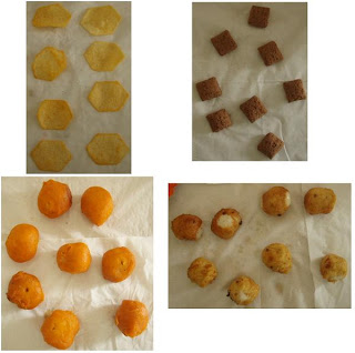
In this activity we are to identify to what class an object belongs to. We do this by extracting relevant features about different samples of the object and comparing its features to a training set. The criteria for membership in a certain class is when its features has a minimum distance to a certain class' representative features obtained by getting the mean of each features of the samples from each class. The classes I used are piatos chips, pillow chocolate filled snack, kwek kwek and squidballs. The images of the objects are shown below:
I chose four features that can be extracted from the objects; normalized area obtained via pixel counting, average value of the red component, ratio of the average value of the green component to the red component, and the ratio of the average value of the blue component to the red component. Since we have only eight samples I used the first four as a training set and the tested the class membership of the training set. The mean feature vectors are shown below:
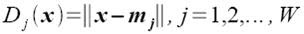
Class membership is obtained by taking the minimum distance between a test's feature to the mean of each feature, following the formula given by Dr. Soriano's pdf file:
Using the features and the above formula, I obtained 15 correct classifications out of 16 samples translating to a 93.75% correct classification.
For the extraction of the parameters of the samples, I performed parametric color image segmentation we learned from activity 16. Afterwards, I inverted the segmented image, performed the morphological closing operation and multiplied it to the original colored image to obtain a colored segmented image. I used excel to perform the minimum distance classification, it was tedious but I understand it better if I do it this way :0. The scilab code I used for the extraction of the parameters is shown below:
For this activity I grade myself 10/10 since I was able to get a relatively high correct classification percentage.
Ed David helped me a lot in this activity. Special thanks to Cole, JM, Billy, Mer, Benj for buying the samples for this activity.

I chose four features that can be extracted from the objects; normalized area obtained via pixel counting, average value of the red component, ratio of the average value of the green component to the red component, and the ratio of the average value of the blue component to the red component. Since we have only eight samples I used the first four as a training set and the tested the class membership of the training set. The mean feature vectors are shown below:

Class membership is obtained by taking the minimum distance between a test's feature to the mean of each feature, following the formula given by Dr. Soriano's pdf file:

Using the features and the above formula, I obtained 15 correct classifications out of 16 samples translating to a 93.75% correct classification.
For the extraction of the parameters of the samples, I performed parametric color image segmentation we learned from activity 16. Afterwards, I inverted the segmented image, performed the morphological closing operation and multiplied it to the original colored image to obtain a colored segmented image. I used excel to perform the minimum distance classification, it was tedious but I understand it better if I do it this way :0. The scilab code I used for the extraction of the parameters is shown below:
For this activity I grade myself 10/10 since I was able to get a relatively high correct classification percentage.
Ed David helped me a lot in this activity. Special thanks to Cole, JM, Billy, Mer, Benj for buying the samples for this activity.
Subscribe to:
Posts (Atom)