Activity 19: Probabilistic Classification

In this activity, we again classify different objects like what we did in activity 18. Only this time we perform linear discrimination analysis. It mainly assumes that our classes are separable by a linear combination of different features of the class. Class membership is attained for when a certain sample has minimum error of classification. A detailed discussion is given in Linear_Discrimant_Analysis_2.pdf by Dr. Sheila Marcos. The samples I used for this activity are piatos(class 1) and pillows (class 2). The features I used are: normalized area obtained via pixel counting, average value of the red component, ratio of the average value of the green component to the red component, and the ratio of the average value of the blue component to the red component. These parameters are obtained using the procedure described in my earlier post for activity 18. The first four samples are used as training set and the last four are used as the test set.


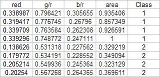
Using the above training set and the methods described in the provided pdf file, we can compute for the covariance matrix given below:

0.0062310 0.0087568 0.0012735 0.0226916

0.0087568 0.0129916 0.0019430 0.0329768

0.0012735 0.0019430 0.0005591 0.0042263

0.0226916 0.0329768 0.0042263 0.0876073

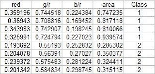
The test set is given below:


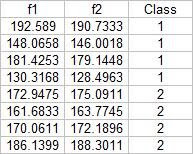
From this test set, the computed discrimant values are:

From these result it is obvious that I was able to obtain a 100% correct classification. I also tried this with a different sample combination (pillows vs squidballs) and I still got 100% correct classification. The following is the code I used:

-----------------------------------------------------------------------
chdir("C:\Users\RAFAEL JACULBIA\Documents\subjects\186\activity19");
x = [];
y = [];
x1 = [];
x2 = [];
u1 = [];
u2 = [];
x1o = [];
x2o = [];
c1 = [];
c2 = [];
C = [];

n = 8;
n1 = 4;
n2 = 4;

x = fscanfMat("x.txt");
y = fscanfMat("y.txt");
test = fscanfMat("test.txt");

x1 = x(1:n1,:);
x2 = x(n1+1:n,:);

u1 = mean(x1,'r');
u2 = mean(x2,'r');
u = mean(x,'r');

x1o(:,1) = x1(:,1) - u(:,1);
x1o(:,2) = x1(:,2) - u(:,2);
x1o(:,3) = x1(:,3) - u(:,3);
x1o(:,4) = x1(:,4) - u(:,4);
x2o(:,1) = x2(:,1) - u(:,1);
x2o(:,2) = x2(:,2) - u(:,2);
x2o(:,3) = x2(:,3) - u(:,3);
x2o(:,4) = x2(:,4) - u(:,4);

c1 = (x1o'*x1o)/n1;
c2 = (x2o'*x2o)/n2;

C = (n1/n)*c1 + (n2/n)*c2;

p = [n1/n;n2/n];
class = [];
for i = 1:size(test,1)
f1(i) = u1*inv(C)*test(i,:)'-0.5*u1*inv(C)*u1'+log(p(1));
f2(i) = u2*inv(C)*test(i,:)'-0.5*u2*inv(C)*u2'+log(p(2));
end

f1-f2

------------------------------------------------------------------------


I proudly grade myself 10/10 for getting it perfectly without the help of others. I also consider this activity one of the easiest because of the step by step method given in the provided file.