Activity 17: Basic Video Processing

In this activity, we are to analyze a video clip. The video clip we will analyze is a simple kinematic experiment and we are to extract certain physical parameters of the experiment and confirm the results analytically. To analyze the video, we need to separate its frames then on this frames we can apply the image processing techniques we have learned so far in the course. The experiment we designed is a simple rolling disk on an inclined plane. An animated gif of the set of images is shown below (video was cropped before images were extracted).


Our goal is to extract the acceleration of the object along the incline. First, we need to segregate the region of interest (ROI) from the background. From our previous lessons, we have two choices of image segmentation, color and binary. Since the video does not really contain important color information, I chose to perform binary image segmentation. The crucial step in this method is the choice of the threshold value. For this activity I found that a threshold value of 0.6 produced good results. However, the a good segmentation was still not achieved since the reflection of light in some parts of the image caused the color of the ramp to be unequal. A gif image of the result after thresholding is shown below:


Clearly, this is not what we want so I performed opening operation using a 10x5 structuring element both to further segregate the ROI from the background of the image and to make the edges of the ROI smooth. The resulting set of images is shown below:



Now we can track the position of the ROI in time. The position over time in pixels can be obtained from the average value of the x pixel position per image. Distance per unit time where distance is in pixels and time is in frames. The conversion factor we obtained is 2mm/pixel and from the video the frame rate is 24.5fps. After conversion I was able to obtain 0.5428m/sec^2.
Analytically, from Tipler, the acceleration along an inclined plane of a hollow cylinder is given by a = (g*sin(theta))/2, where theta is the angle of the incline, for our case theta = 6degrees. Using the formula we get 0.5121m/sec^2. This translates to roughly 5.66% of error. The scilab code I used is given below:

------------------------------------------------------------------------------
chdir("C:\Users\RAFAEL JACULBIA\Documents\subjects\186\activity17\hollow");
I = [];
x = [];
y = [];
vs=[];
ys = [];
xs = [];
as=[];
se = ones(10,5);
se2 = im2bw(se2,0.5);
for i = 6:31
I = imread("hollow" + string(i-1) + ".jpg");
I = im2bw(I,0.6);
I = dilate(erode(I,se),se);
imwrite(I , string(i)+ ".png" );
I = imread( string(i) + ".png");
[x,y] = find(I==1);
xs(i) = mean(x);
ys(i) = mean(y);
end
ys = ys*2*10**(-3);
vs = (ys(2:25)-ys(1:24))*24.5;
as = (vs(2:24)-vs(1:23))*24.5;
-------------------------------------------------------------

I grade myself 9/10 for this activity for not getting a fairly high error percentage.
Collaborators:
Ed David
JM Presto

Activity 16: Color Image Segmentation

The objective of this activity is to "segment" or select a region of interest from an image according to its color. To do this, we have to transform the RGB space into normalized chromaticity coordinates (NCC). We do this obtaining this by dividing each pixel by the sum of the RGB values in that pixel. Afterwards, the chromaticity can easily be represented by two color channels r and g since b = 1-r+g. The image used and the test image is shown below:

OBJECT

TEST IMAGE

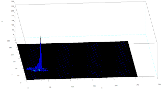
Two methods are used in this activity, non-parametric and parametric. Parametric segmentation is done by determining the probability that a region belongs to the region of interest. In particular, a gaussian probability distribution function is assumed. For non-parametric segmentation, the frequency value of the pixel in the histogram itself is used to backproject the value for that pixel. The two dimensional histogram of the original image test image is shown below:
The x-axis corresponds to the R channel, the y-axis corresponds to the G channel and the z axis corresponds to the frequency. From the figure, it can be seen that the region where the frequency is highest is at the blue region as expected.

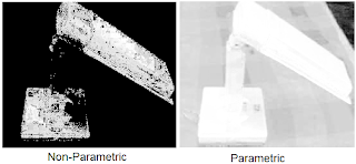
The following are the results of the color segmentation:

It can be seen from the images that parametric segmentation looks better as it was able to approximate the general shape of the blue parts of the lamp are well separated from the other colors. However, the non-parametric segmentation is very accurate in the sense that slight changes in the shade of blue in the image is no longer considered blue. This is easily observed in the post of the lamp since in this part the shade is darker than the top parts.

----------------------------------------------------------------------------------------------
----------------------------------------------------------------------------------------------
Scilab Codes:
Parametric
I = imread("lamp_section.jpg");
orig = imread("lamp_orig.jpg");
av = I(:,:,1)+I(:,:,2)+I(:,:,3);
r = I(:,:,1)./av;
g = I(:,:,2)./av;
b = I(:,:,3)./av;

av2 = orig(:,:,1)+orig(:,:,2)+orig(:,:,3);
r2 = orig(:,:,1)./av2;
g2 = orig(:,:,2)./av2;
b2 = orig(:,:,3)./av2;

r = r*255;
g = g*255;
frequency = zeros(256,256);
sizer = size(r);
for i=1:sizer(1)
for j=1:sizer(2)
x = abs(round(r(i,j)))+1;
y = abs(round(g(i,j)))+1;
frequency(x,y) = frequency(x,y)+1;
end
end
//imshow(log(frequency+0.0000000001));

r = r/255;
g = r/255;

mr = mean(r);
devr = stdev(r);
mg = mean(g);
devg = stdev(g);

pr = (1/(devr*sqrt(2*%pi)))*exp(-((r2-mr).^2)/2*devr);
pg = (1/(devg*sqrt(2*%pi)))*exp(-((g2-mg).^2)/2*devg);

prob = pr.*pg;
prob = prob/max(prob);
scf(0);imshow(orig);
scf(1);imshow(prob,[]);
-------------------------------------------------------------------------------------------------
Non Parametric:
I = imread("lamp_section.jpg");
orig = imread("lamp_orig.jpg");
sizeO = size(orig)
av = I(:,:,1)+I(:,:,2)+I(:,:,3);
r = I(:,:,1)./av;
g = I(:,:,2)./av;
b = I(:,:,3)./av;

av2 = orig(:,:,1)+orig(:,:,2)+orig(:,:,3);
r2 = orig(:,:,1)./av2;
g2 = orig(:,:,2)./av2;
b2 = orig(:,:,3)./av2;

r = r*255;
g = g*255;
frequency = zeros(256,256);
sizer = size(r);
for i=1:sizer(1)
for j=1:sizer(2)
x = abs(round(r(i,j)))+1;
y = round(g(i,j))+1;
frequency(x,y) = frequency(x,y)+1;
end
end
scf(0);imshow(log(frequency+0.0000000001));

r2 = r2*255;
g2 = g2*255;
seg = zeros(sizeO(1),sizeO(2));
sizer2 = size(r2);

for i = 1:sizer2(1)
for j = 1:sizer2(2)
x = abs(round(r2(i,j)))+1;
y = round(g2(i,j))+1;
seg(i,j) = frequency(x,y);
end
end

scf(1);imshow(log(seg+0.000000000001),[]);
scf(2);imshow(orig);
-------------------------------------------------------------------------------------------------
-------------------------------------------------------------------------------------------------

I will give myself a grade of 10 for this activity since the objectives were met and the results are interesting.
Collaborator:
Ed David